Cost-effective genomics analysis

On-demand computing, often known as “cloud computing” provides access to the computing power of a large data center without having to maintain an in-house high performance computing (HPC) cluster, with attendent management and maintenance costs. As even the most casual observers of the tech world will know, cloud computing is growing in any many sectors of the economy, including scientific research. Cheap “computing as a utility” has the potential to bring many large-scale analyses within reach of smaller organizations that may lack the means or infrastructure to run a traditional HPC. These organizations or individuals could include smaller clinics, hospitals, colleges, non-profit organizations and even individual independent researchers or groups of researchers. But beyond the industry enthusiasm, how much can cloud computing really help enable low-cost scientific analyses?

There is now a veritable smorgasbord of offerings from many different vendors, but the big players are Amazon Web Services (AWS), and more recently Google Cloud Engine (GCE). Each cloud provider has different tiers of computing options and different cost structures, but many feature the concept of lower-cost “transient” nodes where the cost per hour (or part thereof) of particular computing node is set by a market mechanism, similar to the way “spot” electricity pricing works. The user can then set a “bid”, and has access to that computing node until the spot price rises above the bid. In the world of AWS Elastic Cloud Computing (EC2) these nodes, or machines, are known as “spot instances”.

A “spot” in the cloud

Having access to a cheap set of nodes without the overhead of a typical HPC, can enable many low-cost scientific analysis. But cloud computing is not a panacea. One has to account for the potential for such transient instances to be lost by a sudden increase in spot pricing (resulting in the “pulling out the plug” on a node), and ensuring that interrupted processes can be resumed smoothly. There is also the additional overhead of ensuring that any analysis and data computations are actively stored for long enough that any individual piece of large analysis can be resumed without repetition.

For long compute-intensive scientific workflows such as the identification of variants in whole genome data, or identification of patterns in machine learning, these are crucial issues. Further, is there a best mix of individual analyses to run, given a certain fixed computing resource; or, given a set of analyses, what is the best set of computing resources?

Cost-effective exome and whole-genome variant calling

In a collaborative project based out of the Laboratory for Personalized Medicine and the Wall Lab, we set out to answer some of these questions in the context of the identification of variants such as single-nucleotide polymorphisms (SNPs) and insertion-deletions (indels) in Illumina whole-genome shotgun sequencing data. We wanted know: given a fixed set of computing nodes, what is the right number of individual genomic or exomic data sets that would minimize the overall cost, whilst simultaneously keeping the run-time of the process reasonable? To do this, we used a 21 node cluster, where we kept at least one master node up at all times (in AWS-speak a node with guaranteed availability is, perhaps a bit confusingly, called an “on-demand” node), but all the remaining nodes were “spot”.

Compact descriptions of complex workflows in Python

We created a Python-based pipeline, GenomeKey, that implemented the GATK (Genome Analysis Toolkit) “best practices” for whole genome and exome variant calling on multiple genomes (or exomes) running simultaneously on this 21-node cluster (full details are in our just-published BMC Medical Genomics paper). This pipeline, in turn, used the COSMOS workflow system to manage the entire run. This workflow management system runs on the main node and keeps track of all the myriad jobs in the system (whole genome variant analysis has many individual jobs many of which can run in parallel). For example, if a node goes down, COSMOS will wait and respool that job once a new machine is available.

Just to give a flavor of what this looks like in practice, here is the top-level Python code using the COSMOS primitives that completely describes the overall variant-analysis workflow (full code has been released under the open-source MIT license and can be found in the GenomeKey GitHub repository):

hc_pipeline = sequence_(
 sequence_( add_([INPUT(b, tags={'bam':sample_name})], stage_name="Load BAMs"), split_(bam_bwa_split, pipes.Bam_To_BWA)),
 reduce_split_(indelrealign_reduce, [chrom], pipes.IndelRealigner),
 map_(                    pipes.MarkDuplicates),
 reduce_(['bam','chrom'], pipes.BaseQualityScoreRecalibration),
 map_(                    pipes.HaplotypeCaller),
 reduce_(['chrom'],       pipes.GenotypeGVCFs),
 split_([glm, skip_VQSR], pipes.VariantQualityScoreRecalibration, tag={'vcf':'main'})
)

In the above, the primitives in bold such as add_, split_, map_, reduce_ follow the map-reduce programming model which will be familiar to users of Hadoop and other systems. The actual analysis stages such as MarkDuplicates, HaplotypeCaller, and refer to individual pieces in the GATK best practices workflow (further implemented by individual Python methods in GenomeKey). Again, detailed descriptions are in the paper and the GitHub repo, but the main point here is that a workflow can be fully described at a high-level in a very compact form.

Creating a StarCluster: deploying remotely from a terminal

StarCluster makes it simple to create and manage EC2 clusters from a terminal application, e.g. on MacOS X or Linux. After editing a simple configuration file, StarCluster can remotely configure and launch a cluster with any combination of instance types and spot-price bids. Again, just to give a sense of how this is done, below we show an example StarCluster configuration file for one particular set of runs of our 21-node cluster. This particular configuration creates 4 of the 21 on-demand nodes (including the master node) to be part of the GlusterFS shared filesystem (see the StarCluster manual for a complete description of each of the options).

[cluster clustername]
KEYNAME = id_clusterkey
CLUSTER_SIZE = 4
CLUSTER_USER = ubuntu
CLUSTER_SHELL = bash
NODE_IMAGE_ID = ami-5bd1c832
NODE_INSTANCE_TYPE = cc2.8xlarge
DISABLE_QUEUE=True
MASTER_IMAGE_ID = ami-5bd1c832
MASTER_INSTANCE_TYPE = cc2.8xlarge
AVAILABILITY_ZONE = us-east-1e
PLUGINS = sge, sge_plus
PERMISSIONS = ssh, http

Once the cluster is launched the ‘addnode’ function can be used to add, say, 17 extra nodes with a spot-bid of $0.50 with the following command:

$ starcluster addnode [clustername] –n 17 –b 0.50

Finding sweet spots

We then downloaded a number of publicly available whole genome datasets (mostly from the 1000 Genomes Project), along with some additional datasets, all in BAM format, and pushed them through our pipeline on a 21 node cluster. So what did we find?

1. One of the first things we discovered is that spot instances were pretty reliable and can make a big difference in the price. For a whole genome, use of spot reduced the cost from around $588 to $109. Setting the bid price, turned out to be a bit of an art, for example spot pricing was unpredictable particularly during sales periods (Christmas, Black Friday etc.), and in some cases the per-hour cost for spot instances exceeded the per-hour on-demand. But by monitoring the average spot prices over a month or so, we were able to set the bid price at approximately $0.5. With these bid prices we rarely lost nodes during a run, but even in those cases, we could recover and complete the runs. Some of these runs were done in 2014, so specific prices will most have likely changed in the interim.
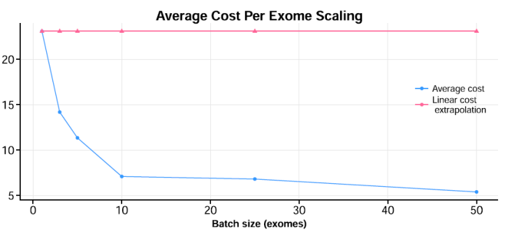
2. Given our fixed number of nodes, we were interested in finding a “sweet-spot” between running too few exomes (or genomes), where you run the risk of wasting resources, and between running too many, where overall throughput could get “gummed up” with larger bottlenecks in I/O or network transfers, reducing overall runtime. To find this spot, we created multiple “batches” in increasingly larger numbers. For exomes, specifically, we found somewhere it between 10-15 exomes (see below). This is just a heuristic, as it will depend a lot on the input datasets.benchmarking

1. The number of nodes participating in managing the storage of the intermediate results between the pipeline stages made a big difference. As noted above, we used a GlusterFS shared volume system, initially using 2 nodes, when we increased this to 4 nodes, we found the overall runtime for 25 exomes dropped from about 20 hours to ~11.5 hours. The overall data transfer rates for particular stages were around two and a half times faster with the 4 node setup.

There are a number of other important technical optimization issues detailed further in our paper, but the main take-home message is this: the cost of performing large-scale analyses such as whole-genome variant identification is dropping significantly and is now within reach of many smaller players. Setting up and running workflows is considerably easier with systems such as GenomeKey, but challenges remain in making these systems even easier to use, and there many new efforts growing around this space.

On-demand computing + open source = enable open and independent science?

Stepping back from the technical advances in the paper, what larger lessons can we draw from these overall cloud-based approaches? New large-scale scientific projects, like NIH’s Precision Medicine Initiative, as well as smaller and medium size clinics and hospitals will obviously benefit from the increasing cost-effectiveness of on-demand computing to process complex human genomic datasets. Cloud services that store and analyze patient’s genomic data raises obvious privacy and security concerns that need to be addressed. AWS and GCE have both made steps towards becoming compliant with U.S. Health Insurance Portability and Accountability Act (HIPAA), but given the rapid pace of technology and law in this area, keeping data secure and private will warrant continual vigilance.

However, the availability of cheaper computing, coupled with advanced open-source workflow tools like GenomeKey could be even more significant within open-science, and smaller-scale research outside human genomic research and larger research institutions. For example, there are many open datasets being generated in many research areas outside the traditionally well-funded biomedical area, including evolutionary and organismal biology, ecology, oceanography, complex adaptive systems and others. Although the continual reduction in cost for cloud-based scientific research will depend on the computing utility market remaining dynamic and competitive, with no one player dominating. Twinning open-source tools for analyzing these datasets with cheap computing, could really propel smaller teams of researchers, individual independent scholars, or citizen scientists to ask many interesting scientific questions not currently being examined in larger research enterprises.

This post is a joint blog post written with Alex Lancaster. Originaly posted on biosysanalytics

For more details, read the paper at BMC Medical Genomics and the COSMOS and GenomeKey website.